
Before we start, a very Happy New Year to all of you from MachineLearningSchool. Everyone might have started acting upon their resolutions already and so are we. Posting articles more frequently is one of our goals this year. That being said, let’s start from where we left off in the previous article. We explained the two main types of machine learning problems, namely regression and classification, and went on to demonstrate them with examples. In this article, we will try to cover one of the widely used algorithms in machine learning, Decision Trees and demonstrate how they can be employed to solve classification problems (applications in regression domain to be discussed in future articles). The fact that we subtly introduced the concepts behind this algorithm, in the previous article, might come as a pleasant surprise. As we move forward, just take a note a Decision Tree is interchangeably referred to as DT.
Trees and Fruits
Remember in the last post when we asked you to imagine to be blindfolded and guess whether the fruit was an apple or an orange? It was a simple classification problem. So how did we proceed? We asked questions about the color, size etc. of the fruit. Well, in simple terms, this is exactly how a DT works. Imagine it to be a talking box which keeps on inquiring about the “features” (explained in the previous article) of the unknown fruit till it is confident about the class (i.e. apple or orange). Also, the next question to be asked, by this talking box, depends upon the answer received to its previous question.
But then you must be wondering why the name Decision Tree was chosen. It resembles the inverted structure of a biological tree and just like it, a DT too has a root, leaves and branches. And like in the above case of deciding whether the fruit is an apple or an orange, DTs are used to arrive at a decision, by asking the right questions, given a task. Hence the name Decision Tree. There you go. Think of it as a talking tree now.
Let’s get back to the fruit classification problem. The figure below demonstrates a simple decision tree that can be used to classify a fruit as an apple or a lemon (orange is replaced for simplicity purpose).

Doesn’t it look like one of those flowcharts that we encounter frequently? Doesn’t it look like an inverted tree? What can you make out from the figure? It represents that if the color of the fruit is green or yellow, then it is a lemon and an apple if it’s red. But, as you might have guessed, this tree might not always give correct results as some apples can be green too. To improve the classification accuracy (i.e. the right guesses), the tree needs to ask more questions about the “features” of the fruit like the size, taste etc. Let’s add in the size feature and see how the tree looks like.

Now, even if the color of the unknown fruit is green, the tree can tell if it’s an apple or an lemon with more confidence since it asks a question about the size too. As mentioned earlier, the next question i.e. regarding the size of the fruit is only put forward if the answer to the previous one, about the color, is green.
Let’s learn more about the DT terminology. The oval shapes in the tree, where the questions about features are asked, are called nodes. What comes at the top if you invert a tree? Root, right? Similarly, the first node (or the first question) in a DT is called the root. The lines carrying the information about the features (or the answers) between the nodes are called branches. What comes at the end of a branch? A node (which might split out into more branches) or a leaf node (which doesn’t split further into branches because when did branches ever come out leaves?). These leaf nodes give out the decision taken by the tree based upon the answers to it’s questions i.e. apple or lemon in this case. A DT which is used to solve a classification problem is called a Decision Tree Classifier. Now that you have a fair idea about DTs and how they can be used for classification, the next part is to figure out how machine learning fits into the picture.
Building the Decision Tree
You know that a DT asks questions but how does it know which questions to ask, when to ask, when to stop asking questions i.e. to give the final verdict and how are the final verdicts chosen. All that you generally have is the raw data but the algorithm behind a DT is clever enough to figure out the details by itself. This might be a little confusing now but it will become clear when explained in context of the above example (with a small modification).
Assume that you own a fruit orchard which yield both apples and lemons. You need to pack the fruit into cartons before selling them to the local market. But there is a problem here. The fruit are always mixed before they reach your warehouse. So you need a quick way to segregate the fruit and pack them separately. After much thinking, you figure out that manually achieving this task is both time consuming and costly. So you turn towards machine learning since you remember that this is but a simple classification problem. You buy a robot, which can determine the color and size of the fruit (we will explain the image processing algorithms which makes this possible, in our upcoming posts on computer vision) and ask it to get this job done in the shortest possible time. The manufacturer specifies that each process, i.e. determining the color and the size of the fruit, takes the same non-negligible amount of time (obviously faster than a human being). So it is obvious that finding out both the color and shape will take more time than finding either one of them. Listening to your end objective, the robot tells you that although it can see the fruits moving on the conveyor belt, you need to teach it how an apple and a lemon look like.
So you select a batch of, say, 1000 fruits, 500 of each class i.e. apples and lemons, and start recording the features, i.e. the color and the size manually, while noting down whether it is a lemon or an apple too. For simplicity, we have assumed that all the lemons which grow in the orchard are green in color and the data is large enough to capture the characteristics of the fruit that grow in the orchard. You handover the data (shown below) to the bot.
| Color/Size | Big | Small |
| Red | (200 apples, 0 lemons) | (200 apples, 0 lemons) |
| Green | (100 apples, 0 lemons) | (0 apples, 500 lemons) |
What does the data say? Out of the 500 apples –
a) 200 are big and red in color
b) 200 are small and red in color
c) 100 are big and green in color
And all 500 lemons are small and green in color.
So, how will the bot move forward to classify the fruits? How will it use the data? It tries to build a Decision Tree. The first step would be to choose between the questions to ask at the root node i.e. question about the color or the size, since there is more than 1 question that can possibly be asked. So how do we choose between the question about color and size. Let’s draw the possible structures of the Decision Tree based on the first question. They are as shown below.
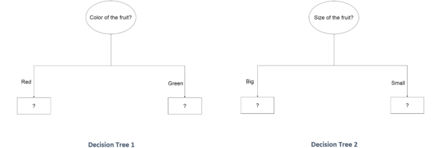
How does the bot know which configuration is better suited for the classification job? And why did I use a question mark at the leaf nodes? How will the tree decide the outputs at these leaf nodes? Well, this is where the data collected earlier comes in handy. The bot feeds each of the 1000 samples and sees how well the trees are performing.
Passing the 1000 fruit samples to Decision Tree 1, we collect the following results at the leaf nodes.

This tells us that if the color of the fruit is red, then it should definitely be an apple because there exists no red colored lemons as per the data. So, the tree learns this rule ( i.e. if the color of the fruit is red then it is an apple), from the data, and set the output of this leaf node to apple. No further questioning is needed. These kind of leaf nodes, where there is no confusion about the output, are called pure nodes. What happens if the color of the fruit is green? We can see that the 100 green apples can’t be differentiated from the lemons by the tree. So the DT is not confident about the output at this leaf node because the tree cannot definitely say that if the color of the fruit is green, then it is a lemon (or an apple) based on the data. There are two possibilities in such case. The first one being setting the output of the leaf node to the majority class present i.e. lemon in this case because there are 500 green lemons when compared to only 100 green apples. In other words, the tree is at least more confident that a green fruit might be a lemon rather than an apple. These kind of leaf nodes generated, even if there is confusion regarding the class, by taking majority voting are called impure nodes. The other possibility is to ask another question at this node which tries to bring down the confusion about the class. This explains the parts “when to stop asking questions i.e. to give the final verdict” and how are the final verdicts chosen” that I mentioned earlier. After this process, Decision Tree 1 looks like (assuming we decide to ask more questions if the fruit is green):

Now if we pass the 1000 fruit samples again to DT 1, it would correctly classify the 400 apples which are red in color and subject the 600 fruits (100 apples + 500 lemons) which are green, to further questioning.
Repeating the same process with Decision Tree 2, we collect the following results at the leaf nodes.

This tells us that if the the fruit is big, then it should definitely be an apple because there exists no big lemons as per the data. So, the tree learns this rule ( i.e. if the size of the fruit is big then it is an apple), from the data, and set the output of this leaf node to apple. From the previous definition, this leaf node is a pure node too. But what happens if the fruit is small? We can see that the 200 small apples can’t be differentiated from the lemons by the tree. So the DT is not confident about the output at this leaf node because the tree cannot definitely say that if the fruit is small, then it is a lemon (or an apple) based on the data. This is an impure node and the majority vote favors lemons because there are more small lemons than small apples. After this process, Decision Tree 2 looks like (assuming we decide to ask more questions if it’s a small fruit):

Similarly if we pass the 1000 fruit samples again to DT 2, it would correctly classify the 300 apples which are big and subject the 700 fruits (200 apples + 500 lemons). which are small, to further questioning.
The choice of the first question to be asked at the root node is yet to be decided. Let’s assume that the time taken for either of the color or the size measurement by the robot is ‘x‘ seconds. We try to calculate the average time taken by each DT to process a fruit.
In case of the Decision Tree 1, all of the 600 green fruits (100 apples + 500 lemons) should be asked a further question (i.e. about the size) to resolve the classification confusion.
Time for first question for 1000 fruits  = 500x + 500x  (i.e. for 500 apples and 500 lemons)

Time for second question for 600 fruits  = 100x + 500x  (i.e. for 100 apples and 500 lemons)

Average time taken =  (Time for first question + Time for second question ) / (No. of fruits) = 1600x/1000 = 1.6x
In case of the Decision Tree 2, all of the 700 small fruits (200 apples + 500 lemons) should be asked a further question (i.e. about the color) to resolve the classification confusion.
Time for first question for 1000 fruits  = 500x + 500x  (i.e. for 500 apples and 500 lemons)

Time for second question for 700 fruits  = 200x + 500x  (i.e. for 200 apples and 500 lemons)

Average time taken =  (Time for first question + Time for second question ) / (No. of fruits) = 1700x/1000 = 1.7x
So, we would choose question about the color as the first one since the fruit gets segregated faster in this way as the confusion is reduced to a greater extent by querying about the color first rather than size. This is the fundamental concept behind Information Gain, calculated on the basis of Entropy, which is actually used while deciding the question at each node in a DT. The mathematics behind this will be explained in a later article since we aim to keep this article simple.
As discussed earlier, after choosing the first question about the color, we try to add a new question to the node, when the fruit is green. The only other possible question is about the size of the fruit (since it makes no sense in re-duplicating the question and asking about the color again). After adding the new question and passing on the samples to it, DT 1 looks like this:

By the same logic, we find that the two new leaf nodes are pure and therefore, we can stop asking questions and assign outputs to each of them. From the data, if the fruit is green and big, then it is definitely an apple and if it’s green and small, then it’s definitely a lemon. So, by asking an extra question, when in doubt, the tree clears the confusion about the fruit type when it’s green in color. This little exercise explains the part “which questions to ask and when to ask them” which I mentioned earlier.
The bot generated the Decision Tree Classifier (shown below) based on the data and is now ready to use. Summarizing, this whole process of the tree finding the questions to ask, the order in which to ask them and the outputs to generate based on the answers, from the raw data is called Decision Tree Learning. The raw data (i.e. the 1000 fruit samples) which is used for this purpose is called the training data.

Cutting down the Tree
Let us assume that while observing the features of the 1000 sample fruits, you made a mistake and now the data looks like the following:
| Color/Size | Big | Small |
| Red | (200 apples, 0 lemons) | (200 apples, 0 lemons) |
| Green | (95 apples, 0 lemons) | (5 apples, 500 lemons) |
If you didn’t notice the difference, there are now green apples which are small. Though this mistake doesn’t change the order in which the questions are asked (do the math), it would have an impact on the purity of some of the leaf nodes. The DT, when tested on the training data, would yield the following results:

As you could see, the leaf node at the extreme right is impure because now there are 5 small green apples that can’t be differentiated from lemons. What would be the output at this node now? Based upon our earlier discussions, we could either take the majority vote here and set the output of this leaf node to be lemon (which introduce a scope for error) or ask an additional question if the fruit is small and green. But are there are any valid questions that can be asked at this node now? No, we exhausted all the features (i.e. color and size). So we need to introduce a new feature, for example, allow the machine to taste the fruit via a small hole (just a hypothetical feature). This would resolve the confusion about small green fruits, as shown below:

But how does the tree decide between taking the majority vote or exploring new features? In this case, the choice is to be taken by us, the humans, based on the cost that would be incurred in both cases. For example, if the customers for our fruit are very particular about the orders they receive, we should probably incorporate the taste feature (which would increase the processing time). On the other hand, if the customers are fine with a few discrepancies, we can neglect the small possibility of error and remove the extra node, call the previous node a leaf node with the output as the majority vote decision i.e. lemon. This process is called pruning (in gardening, to prune is to remove the unwanted parts of a plant). In this process, the extra questions asked at the nodes are removed if the information (indirectly accuracy) gain is negligible. Well, insignificant accuracy gain by introducing the extra nodes is one of the reasons pruning is applied on DTs. The other being to avoid overfitting, a term in machine learning you should definitely be aware of.
Let’s lighten up the mood a bit. The only machinery operator at your fruit processing plant is about to retire. Realizing that he is almost irreplaceable, you decide to put up an advertisement to hire someone similar. The ad goes like this:
Wanted: Plant operator. 42 years and 89 days old male with diploma in Mechanical Engineering from ITI Bangalore. Must be 5 ft. 7 in. tall with brown hair, a mole over the right eye. Should suffer from diabetes and have a Redmi Note 3.
These are the exact qualifications and traits of the existing operator but would this ad succeed in getting a good replacement? This a real life example of overfitting. Simply put, overfitting, in the context of DTs, is asking more questions than what is actually needed to take a decision. This would work well with the data in hand but will fail with new unseen data, i.e. we will definitely select the existing operator (if he decides to reapply) based on the ad but would fail in selecting good candidates just because their traits, which are completely unrelated to the job, aren’t matching. So, what would be the opposite of overfitting? Underfitting right? What would it look like? Probably an ad that goes like this:
Wanted: Plant operator. Should have a diploma from ITI Bangalore.
This ad would not fetch a good replacement as it doesn’t look into all the relevant qualifications required. For example, a diploma in Mechanical Engineering might be required to operate the heavy machinery. The solution to avoid the problem of overfitting/underfitting is to ask the right number of relevant questions, not too many nor too less (more on this in upcoming articles).
Looking at Decision Trees in a different way
What if I told you that DTs can be interpreted in a simpler way? For this you need to plot the features on the spatial axes:

So a Decision Tree, effectively, divides the feature space into sub-regions iteratively (till no more questions need to be asked) and assigns each subspace an output (decision). Each subspace represents a node or a leaf in the tree. We could easily visualize it here because there are only two features (2D plot) but it becomes difficult to imagine this subdivision division when the number of features are greater than 3 (i.e. > 3D).
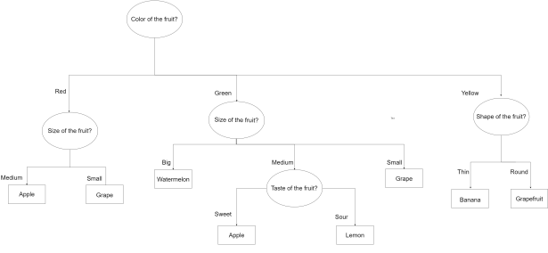
In this article, we tried presenting the concepts of Decision Trees and their application in Machine Learning in an intuitive, non-mathematical way. We are keeping the calculation intensive part of this algorithm for the future posts, in which implementing DTs in different software platforms will also be discussed using openly available data. We will end the article by showing how DTs can be used to solve bigger classification problems, where there are more features and classes (shown below). We will adhere to our promise of keeping the content simple and easily understandable in the future posts too.
Please provide us your feedback about the post and we will keep them in mind while creating new content.
Thanks,
Naveen and Saketh
Disclaimer: This is a personal blog. Any views or opinions represented in this blog are personal and belong solely to the blog owner and do not represent those of people, institutions or organizations that the owner may or may not be associated with in professional or personal capacity, unless explicitly stated
